How many of the top hitters and pitchers at the end of the year were actually drafted? How many of the top hitters and pitchers were not drafted and were picked up during the season? Were hitters or pitchers drafted more accurately? What is the dollar value earned by the players that were picked up during the season? Is there a position of hitter that’s more reliable than other positions?
Have you ever asked yourself draft analysis questions like these?
What follows is a five year analysis (with colorful graphs and an enormous Excel file!) of how accurately our projections in the preseason depict what has actually happened at the end of the season. How well we drafted. What positions yield the best returns. What positions offer the most free loot. And more.
Assumptions You Should Know
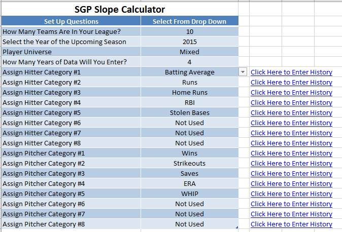
A number of the graphs depend on dollar value earnings for the “top 168″ projected hitters or “top 108″ projected pitchers. The dollar values are calculated using the approach documented in “Using Standings Gain Points to Rank and Value Fantasy Baseball Players” assuming a 12-team league, $260 team budget, 14 hitters (C, C, 1B, 2B, SS, 3B, CI, MI, OF, OF, OF, OF, OF, UTIL), 9 pitchers, and a 70%-30% hitter-to-pitcher allocation. That’s a total of 168 hitters and 108 pitchers.
These top projected players in the preseason were determined using Steamer’s preseason projections for that season (I downloaded the historical projections here).
I suppose using ADP results or expert rankings from the given year might give a better picture of the players that were actually drafted, but then you get into the question of what’s good ADP data, where to get it, what experts to use, league differences, lineup differences, etc.
To Be Clear… The Goal of this Study
The goal of this is not to measure the accuracy of particular experts. It is to determine which positions can we draft and get the most return on our investment. To some extent this is a review of Steamer’s accuracy, but that’s also not my intent. It’s my understanding (tell me if I’m wrong) that there are not significant differences between the top projections systems. So whether we were looking at PECOTA, Steamer, or Marcel projections, we would see similar results.
How Much of a Return Do We Get For Drafting HItters vs. Pitchers?
People have long been telling us to, “Load up on hitters early in the draft”.
“Don’t overspend on pitching.”
“Wait on pitching until most teams already have one.”
I’ve always heard these things. They sounded right. But I can’t say I’ve ever seen the data to support it.
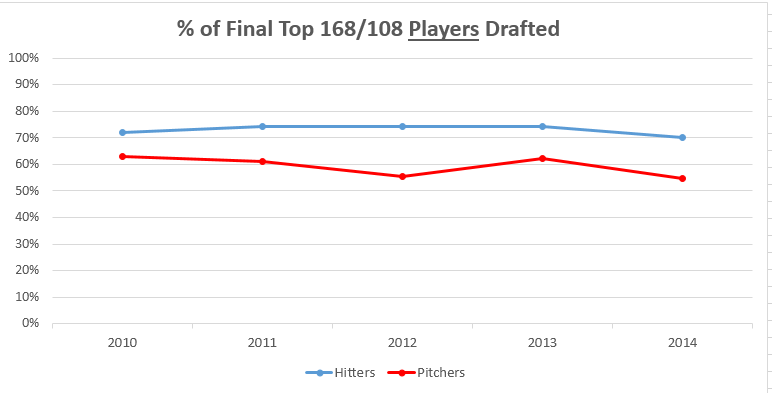
In looking at the chart below it is very clear that we are much better at identifying the top hitters than the top pitchers. The top 168 hitters in the preseason provide about 70% of the dollars earned at the end of the season. For pitchers, it’s more in the neighborhood of 40%.
With results like that it’s very easy to see why the hitter-pitcher split is not 50-50.
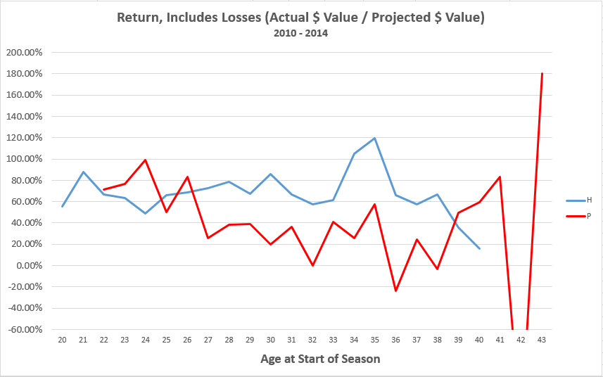
Hitters are safer investments than pitchers. We’ve always been told this, but now you can see it. And things have not changed in the new era of pitching that we’ve been seeing the last few years. If anything, the gap seems to have widened.
![Hitter-Pitcher-Draft-Returns-With-Losses]()
In a draft and hold environment, the return on investment for drafting hitters fluctuates between 65% and 80%. The return on pitchers is much lower, falling roughly between 30% and 50%.
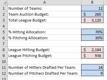
If you’re curious about the math on this, read this paragraph. Otherwise, skip on over this one. Going back to our assumption of a 12-team league where each team has a $260 budget, that gives the league $3,120 to work with. If 70% of that is earmarked for hitters, that means $2,184 of value is allocated to the pool of 168 hitters and $936 is designated for the 108 pitchers. The 70% return on hitters means that we projected who the top 168 hitters would be in the preseason and by the end of the season those same 168 hitters were worth about $1,530 ($2,184 * 70%). So about $654 of value came from hitters that were not drafted.
Why Does That Chart Say “(includes losses)” In The Title?
The calculations above were done in a “draft and hold” scenario, meaning if Cliff Lee is projected as a $20 player prior to the 2014 season and his end of season earnings are a negative $9, he returned a value of -$29. These “losses” can really affect the calculations.
You’re probably thinking, “But not all pitchers (perhaps none) are held on a roster when they’re having a really bad season”. And if a pitcher suffers a season ending injury, they would be cut immediately and also would not end with negative earnings for the season.
A bit further down you’ll see charts for scenarios where losses are eliminated. So instead of negative $9 Lee comes in with just a $0 return.
This scenario of Lee breaking even is a little too optimistic. If a pitcher is struggling and on his way to a negative earning season, it can take weeks or months for us to make that determination. As that time goes by you’ll be accumulating some of those negative earnings on your team.
The true return lies somewhere in between the “no losses” and “includes losses” lines.
How Much of a Return Do We Get at Each Position of Hitters Vs. Pitchers?
We’ve seen that hitters as a group are a greater investment than pitchers. But what about the individual hitter positions?
![Hitter-Position-Pitcher-Draft-Returns-With-Losses]()
Breaking the hitters into different positions, you see a lot of fluctuation in returns, but it’s very clear that drafting any type of hitter is expected to result in higher return on investment than drafting a pitcher.
There’s a lot going on here, but it’s very clear that any position of hitter is a safer investment than a pitcher. Outfield appears to be a very consistent producing position. Rarely the highest in a given season, but steady. SS and 3B fluctuate wildly.
1B might be the overall lowest returning position of all. Prince Fielder, Joey Votto, Chris Davis, Paul Goldschmidt, Billy Butler, Eric Hosmer, Brandon Belt, Mitch Moreland, Kendrys Morales, and Adam Lind really dragged the return down in 2014, while Albert Pujols, Adrian Gonzalez, Joey Votto, Mike Napoli, and Lance Berkman disappointed in 2012.
We’re a long ways from the glory days of Todd Helton, Jason Giambi, Jim Thome, Carlos Lee, Paul Konerko days when 1B seemed like a lock every season.
But We Don’t Have To Draft and Hold.
As I mentioned above, very few of us play in draft and hold leagues. We can replace struggling or injured players that appear to be negative earners.
There’s no way to measure exactly when a player will be dropped. The best we can do is to remove the possibility of a player returning negative earnings. A replacement level player would have earnings of $0.00. So assigning a value of $0 to players that would otherwise have negative earnings makes some sense. If a struggling player is performing at about the same level as available free agents, we would probably hold on to them and hope they can turn it around.
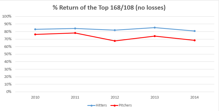
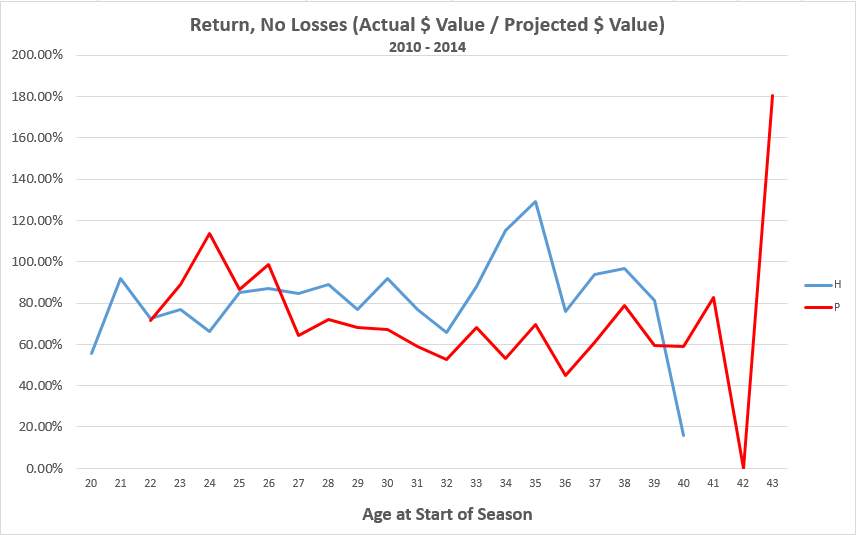
When we remove the possibility of losses, the gap closes. Pitchers come much closer to the results from hitters.
![]()
Part of the reason pitchers return less than hitters is their greater likelihood of suffering season-ending injuries. A pitcher having Tommy John surgery in the first month of the season will surely have negative earnings for the year. But even if we place a restriction that pitcher cannot have negative earnings, they still don’t return as much value as hitters.
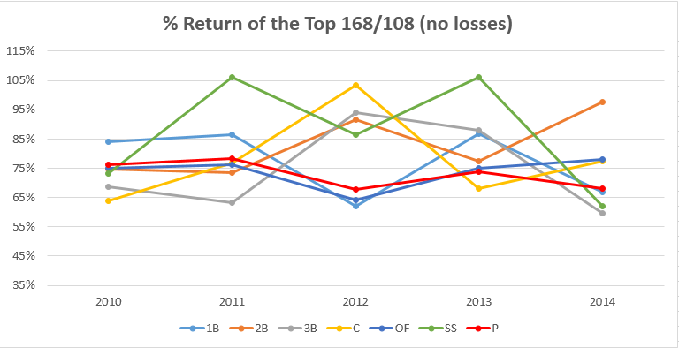
Splitting all hitters into separate positions, pitchers are not usually the worst performing position in any given year. But unfortunately pitchers do look like the worst performing investment
![]()
When the group of all hitters is broken into different positions, pitchers are not the lowest performing group each season, but they are still the lowest performing group overall (although outfielders are surprisingly close!).
The Truth Lies Somewhere in the Middle
We don’t play in draft and hold leagues and there’s not a magic fairy that tells us exactly when to drop a player before he starts earning us negative return. The actual return we can earn for a hitter lies somewhere between the blue lines below. The actual return for a pitcher lies somewhere between the red lines.
![RETURN-HITTERS-PITCHERS-BOTH]()
If we place the “no losses” returns on the same chart as the “with losses” returns, pitchers reap a larger benefit than hitters do. But it’s important to keep in mind that not every negative earning pitcher is due to a season ending injury. Some negative earners are easily dropped because of an injury while others just perform poorly and struggle all season long.
How Much of the End of Season Earnings Were Acquired During the Draft?
Let’s shift gears a bit. Of all the earnings for each position at the end of the year, how much of them were obtained through the draft?
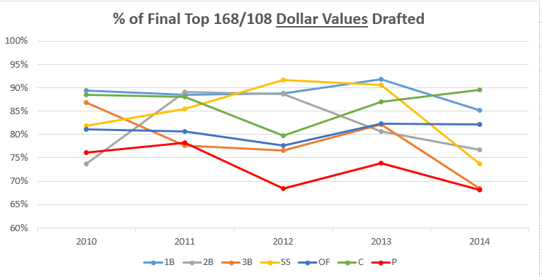
You can see in the chart below that we’re very efficient at drafting all of the earnings from 1B and C. My guess is that’s not a function of us being better at projecting 1B and C. It’s more due to the fact that these positions have a greater percentage of MLB starters drafted than other positions. In a two-catcher league, 24 out of the 30 starting catchers are drafted. First base is similar in that players are drafted to player first 1B, corner infield, or the utility spot.
So even though we saw above that 1B provides a pretty low return (when we allow for negative earnings), we still end up drafting nearly 90% of the value at 1B. This implies that there are not a lot of valuable free agent pickups that come along at 1B.
![Hitter-Position-Pitcher-Percent-of-Dollar-Values-Drafted]()
We’re very good at identifying and drafting the value from the 1B position, meaning little value can be acquired once the season starts. We are less skilled at identifying 2B, OF, and 3B. We’re worst at drafting the top pitchers. It is easiest to find valuable 2B, OF, 3B, and P once the season starts.
How Many of the Top Earning Hitters and Pitchers Were Drafted?
Forget about earnings and dollars for a minute. How many of the top 168 hitters at season’s end were drafted? How many of the top 108 pitchers?
![Hitter-Pitcher-Percent-of-Players-Drafted]()
Acquiring value is what ultimately leads to success, but what about the actual number of players that are drafted? If we draft 168 hitters, approximately 70-75% (118 – 126) of them will be the “top earners” for the year. Of the 108 drafted pitchers, approximately 60% (65) of them will be among the “top earners”
It’s starting to look like any way you slice it, hitters are a more sound investment.
How Many of the Top Position Players and Pitchers Were Drafted?
Let’s break hitters apart into different positions.
![Hitter-Position-Pitcher-Percent-of-Players-Drafted]()
This chart breaks apart the “Hitters” grouping from the graph above. You can see we draft about 70% of the top earning OF for the season (usually 64-68 OF will be drafted in the top 168), or 45-48 actual players. 3B appears to be a volatile position. Some years we are good at identifying the top earners and others we’re not.
This does support the theory I presented above that we draft more 1B and C than other positions so we have a greater chance of getting more of the top players at the position right. The more times you toss a coin, the more heads you’re going to land on.
Another thing that jumps out at me is the significant dip for 3B in 2012. That year we actually did a good job of identifying 3B in the preseason. Miguel Cabrera, Adrian Beltre, David Wright, and Ryan Zimmerman all earned more than projected. Chase Headley was pegged as the 11th best 3B and we caught lighting in a bottle when he earned $27. But we did not see Mark Trumbo, David Freese, Kyle Seager, Pedro Alvarez, Chris Johnson, or Todd Frazier coming.
It’s finally dawned on me why the OF line is so stable in all of these graphs. It’s simply a numbers game. When we draft 60-70 OF each season, that denominator stabilizes because of the larger sample of players at that position. If we were only drafting 14-18 like at 3B, SS, and 2B, the lines would be subject to much greater fluctuation.
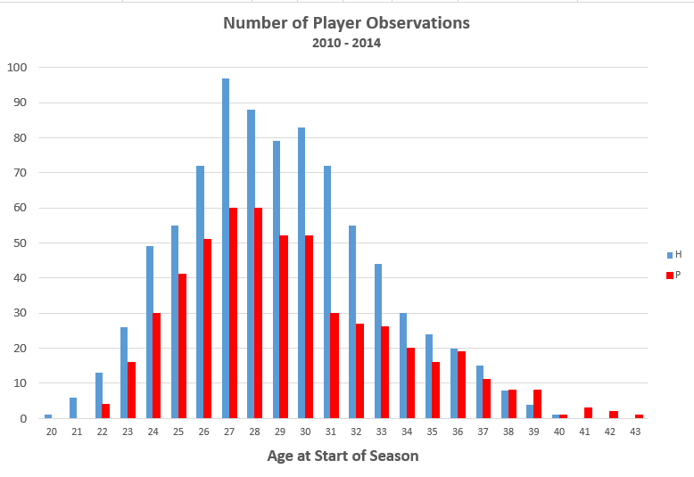
How Many Valuable Players Come Into The League Each Season?
This graph is the exact inverse of the “% of Final Top 168/108 Players Drafted” chart above, but I think it’s helpful to view it from a different perspective. Instead of thinking, “How good at we are identifying the good players in the preseason?”, we might flip it around and wonder, “How many good players are going to be available through free agency once the season starts?”.
This is the concept of “free loot” that I learned of from Peter Kreutzer’s Rotomansguide website (which I highly recommend checking out if you like thinking of the concepts in this post).
![Free-Loot-Not-Drafted]()
Instead of thinking, “How good at we are identifying the good players in the preseason?”, we might flip it around and wonder, “How many good players are going to be available through free agency once the season starts?”.
No surprises here. More pitchers become available through free agency.
Take a serious minute to think about what these numbers mean. Of the nine pitchers you draft, four of them you’ll be completely wrong on. They are not even going to be in the top 108 pitchers at seasons end. Five right. Four wrong.
Of the 14 hitters on your team, you’ll probably only be wrong on four of those too. Ten right. Four wrong.
![Free-Loot-Not-Drafted-Positions]()
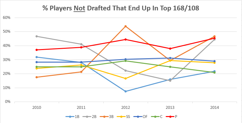
What percentage of players at each position are not drafted and end up being available to acquire during the season?
Percentages can be deceiving at times. So how about the actual number of undrafted players that end up in the top earners.
![NUMBER-HITTERS-PITCHERS-NOT-DRAFTED]()
Percentages are great. But it can be helpful to talk actual numbers. Somewhere between 40-50 positive earning hitters and pitchers will be available through free agency. Keep in mind that this makes pitchers “more likely” to become available because only 108 pitchers are rostered while 168 hitters are.
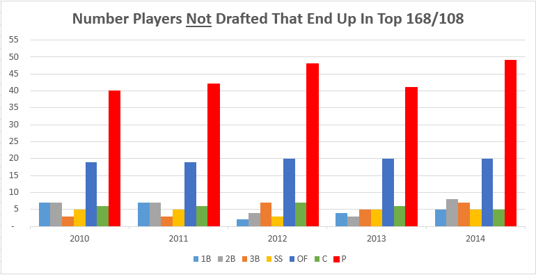
And by position.
![POSITIONS-FREE-LOOT]()
Somewhere in the neighborhood of 40-50 free agent pitchers will earn positive value during the season. Approximately 20 OFs, five C, and five SS will appear.
I’m not sure there is much to take from this. But I figure I’ll show it to you anyways. I think this is largely due to the function of us drafting 108 pitchers, 60-70 OF, and 14-20 players at other positions.
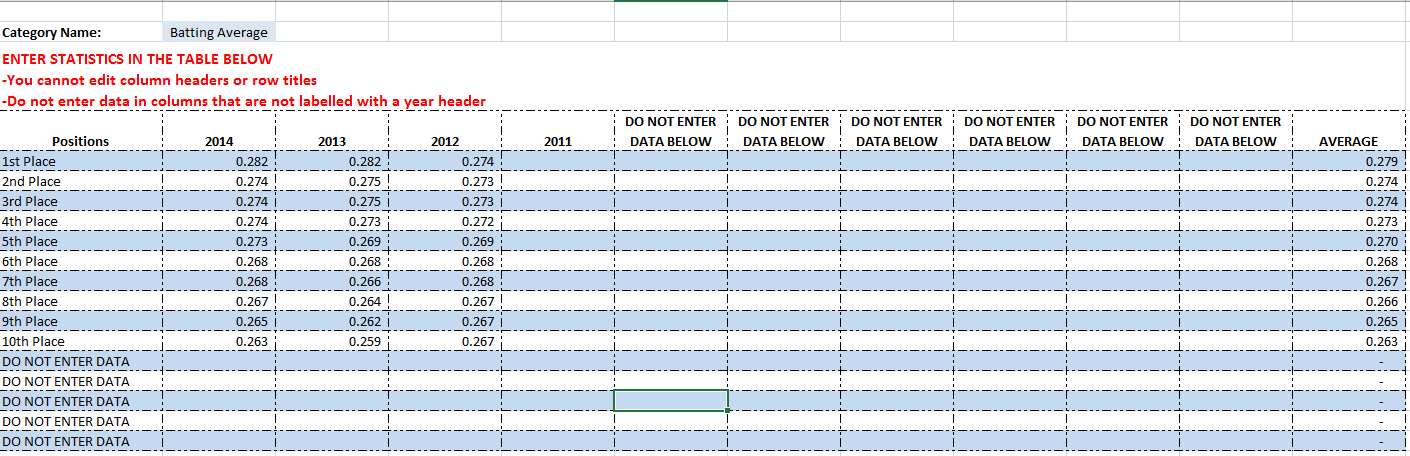
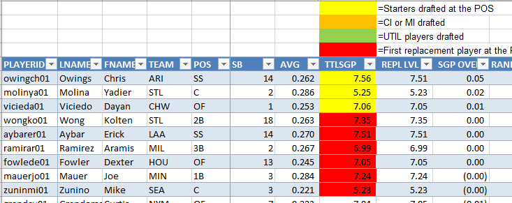
The Data
Unfortunately the Excel file is so large that I can’t post it for you to view online, but you can download the file here (SGP Reliability Research for Download.xlsx). There are tabs for projections and actual stats for hitters and pitchers for each season from 2010-2014. The “SGP Charts and Summarized Data” tab summarizes the returns for each position, each year, and also contains all the graphs above. The “Historical SGP Results” tabs summarize the projection and actual results for each hitter from 2010-2014.![Excel_File_Tabs]()
Conclusions and Takeaways
There is a lot of information to take away from this. But I now have very easy to understand visual proof as to why you are best off delaying on drafting pitchers.
There’s also no truth to the rumor that because pitching has become more dominating in recent years that you need to draft it any earlier. Pitching comes out below hitting in nearly every measure in every season. Even in the “pitcher’s era” we find ourselves in now.
I also realize I need to treat hitters and pitchers with different levels of patience in the season. Looking back, I’ve found myself trying to practice high levels of patience with underperforming pitchers. Given the higher level of turnover in the top 108 pitchers than the top 168 hitters, it’s fine to be less patient with pitchers and more patient with struggling hitters. We’re wrong about four out of every nine pitchers!
Why It’s Important to View Things in Terms of Dollar Values
We don’t all play in auction leagues, but there is still value in converting player statistics into dollar values. If we don’t convert player statistics into some singular number to rank players, the analysis above is not possible. We could just use each player’s standings gain points, but there’s something more meaningful about using dollars. And over time we’ve come to have an understanding of what a $30 or $40 season means.
What Is Left To Be Done?
I’ve answered a lot of questions above. But this has led me to more questions. So the return on ALL hitters is about 70% and the return on ALL pitchers is in the neighborhood of 40%. What’s the return on all $30, $20, and $10 hitters? Pitchers? What about $20 1B versus $20 OF? How does the typical $10 SS pan out when compared to the $10 pitcher? What about 30 year old hitters versus 27 year old hitters?
I’ll get there some day…
What Did I Miss?
Did you see something interesting in the charts above that I didn’t point out or comment on? Let me know in the comments below.
What Do You Want To Know?
What questions were popping up in your head as you read this? Let me know in the comments and I’ll attempt to find the answers.
Thanks for reading. Stay smart.

 If you’re looking for a way speed things up by watching them 1.5 or 2 (double) speed, cutting down the time it takes to watch significantly. Just adjust the settings at the bottom of the video player. Click the cog and change the “Speed to 1.5 or 2.


 There’s not even an existing Excel formula we can use to just pull out the web address. We have to get a little advanced and create our own.

 The new module is where we can “code” the new function. You should notice that a blank white area now appears on the rightportion of the screen. This is where we will place the code.


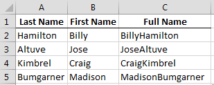
 You can then copy the formula down to the other rows of data.
 TIP: I’m sure there’s an easier way to do it, but the formula I used to get the player ID out of the Razzball addresses is:


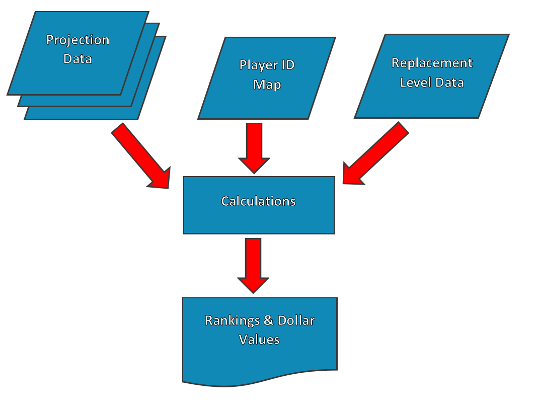
 If you’re not familiar with flow-charting (I’m no expert myself, I had a class in college about 15 years ago about process modelling), there’s something subtle different about the projection data.
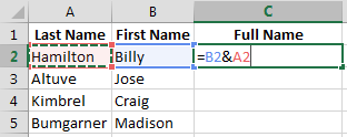
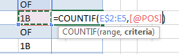
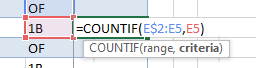
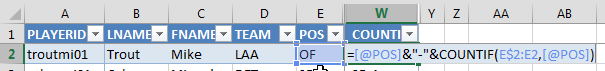
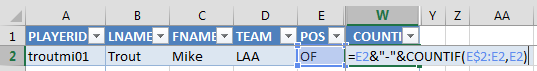


 If you don’t like the Structured Reference notation, you can manually type in “E2″ and get the same result.


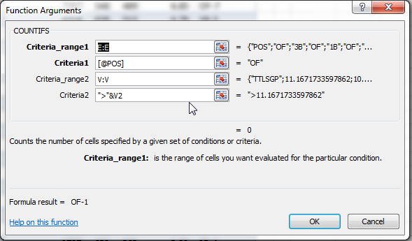
 If you leave this at >[@TTLSGP], you can see that Excel is not able to interpret this.
 Click “OK” to accept the formula as it is.
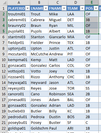
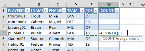
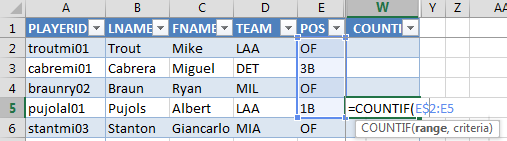
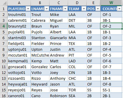
 We actual want Trout’s rank, not how many are higher than him. His rank is first. The second player, Ryan Braun, is evaluating to a 1. But really he’s the second ranked outfielder.


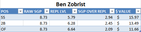
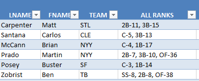 How do we handle the multi-position players like Ben Zobrist and Martin Prado? When a player is eligible to be slotted at 2B, SS, and OF, how do we value that player?
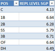


 ” is now available at Amazon.com.
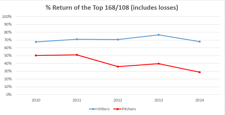


 You can take an Excel file and open it in a second window, allowing you to look at two separate tabs at the same time. This works really well if you have dual monitors. Put one window on monitor A and put a second window on monitor B. I use this for transferring the replacement level information from my hitter ranks tab to my replacement level information table.
 As I mentioned, this post assumes you have already added the named range and data validation drop down listing to select the team that has drafted a player.
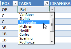
 Then click on the “Insert” tab. Finally, click on the “Pivot Table” button.


 Toward the right of your screen, you should see the list of all fields in your data.

 Notice how the listing of teams also has a “(blank)” item? This would represent any player with nothing in the “Taken” column. Or undrafted players.
 When you drop them, you should see Excel label them as “Sum of [category]” (for example, “Sum of AB”). If you see “Count of [category]”, be patient. We’ll fix that shortly.
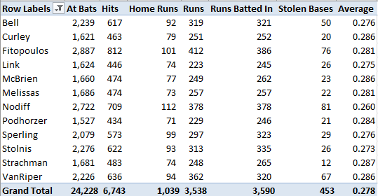
 This screen is where you can customize the description of the column (“Sum of AB” is not a sexy column name) and change from “Count of” to “Sum of”, if necessary.
 Note that you cannot name the column “AB” because that’s the name of a field in the table. That’s why I labelled mine “At Bats”. Sure beats “Sum of AB”…
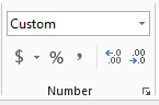
 Then click the “Comma” number style and decrease the decimals two times (to remove the decimals).

 In the “Formula:” field, replace the “=0″ with our calculation of batting average, “=H/AB”. Instead of typing the formula, I recommend double-clicking on the field names for “H” and “AB” (you can type the “=” and “/”).
 Make sure to click “Add” when you’ve given the name and formula calculation.
 Then select the values in this column and increase the decimals three spots so it looks like an actual batting average.
 Once on this tab, click on the “Options” drop down menu all the way to the left of the ribbon (underneath the “PivotTable Name” area). Make sure the “Generate GetPivotData” option is
 Paste the headers below the Pivot Table. Leave a column to the left of the headers (I pasted them in column B, leaving column A open).

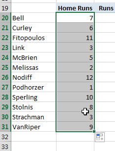
 Your Pivot Table may be positioned slightly different than mine. I’m now going to add a formula to cell B20 (in the image above). Add your formula so that it will calculate the “Home Runs” for the first team.
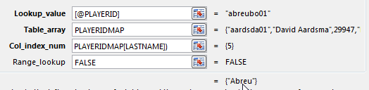
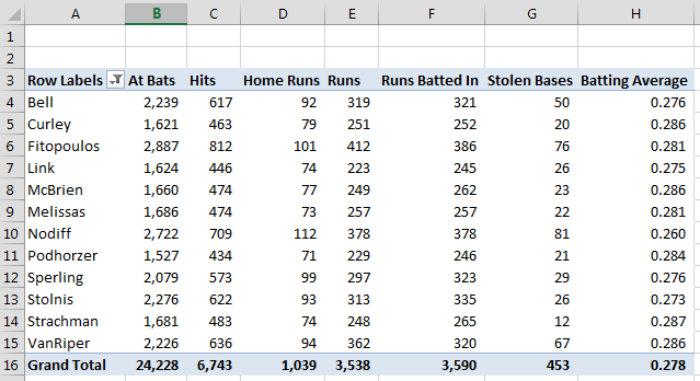 And here are the inputs into the formula.


 Be sure to download both the
  This will download a CSV file to your computer.
 As you download more and more reports from Fangraphs they will be sequentially numbered (1), (2), etc.Open the hitters file in Microsoft Excel first. Right click on the tab and select the option to “Move or Copy…”.
 At the next menu, click the drop down menu. Choose your rankings Excel file (created above) from the drop down list. Then hit “OK”.
 Repeat this step for the pitcher projections.
 It will be important to name your spreadsheet tabs with meaningful names so you can easily keep track of what each of the spreadsheet represents.I will name my tabs “Steamer Hitters” and “Steamer Pitchers”.


 If you’re interested, Smart Fantasy Baseball Blue is custom color 17R, 137G, 183B on the RGB scale.

 Name this sheet “Scoring Settings”.
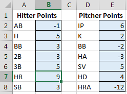
 On your “Scoring Settings” sheet, create a list of the various scoring categories and the point value for each.


 While the Format Painter is still active (you can tell it’s active when you see the paint brush icon next to your cursor), simply click in all the other cells containing scoring point values.
  After you have selected all the point value cells, hit your ESC key to exit the Format Painter.
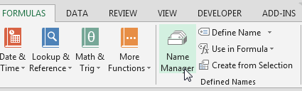
 Then click on the “Formulas” tab of the ribbon and select the “Define Name” button.

 Look over your list of names and make sure you haven’t missed anything.
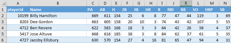

 You will then be prompted to verify the range of cells in the table and that your table has a header row (e.g. Name, AB, H, HR, etc.).
 Check “My table has headers”. Click OK.


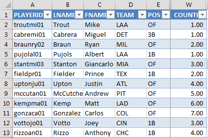
 After you’ve renamed the sheet, type “PLAYERID” into cell A1. This will be a column header for our next step.


 Check “My table has headers”. Click OK.

 If so, click once in the area between the Column “A” header and the Row “1” header (the top left corner of all cells), to select all cells in the entire sheet.


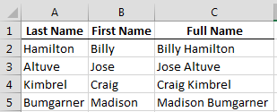
 Then simply double click in cell C2 and change the column name (remember column names are surrounded in [brackets]. So change [LASTNAME] to [FIRSTNAME].).


 You will then be prompted to verify the range of cells in the table and that your table has a header row (e.g. Name, W, L, ERA, etc.).


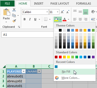
 If so, click once in the area between the Column “A” header and the Row “1” header (the top left corner of all cells), to select all cells in the entire sheet.
 Then click the “Fill Color” icon (looks like a paint can) drop down arrow and choose the “No Fill” option.
 You should now see the proper alternating color scheme.


 Then simply double click in cell C2 and change the column name (remember column names are surrounded in [brackets]. So change [LASTNAME] to [FIRSTNAME].).
 Nerdy Excel talk here, but dragging formulas within tables does not work very well because there’s no way to make the formulas absolute (they want to stay relative as you move them). That’s why I suggest copying and pasting the formula, even if it duplicates and you then need to change part of it.


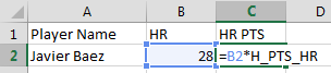
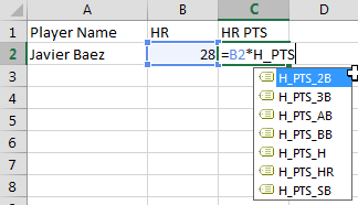
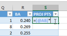 Excel should recognize the name you’re typing and present you with a list of named cells which follow that pattern. Once you see this list you can double-click on the desired name, use your arrow keys to select “H_PTS_AB” and hit TAB to choose it, or just continue typing the full name.
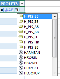 In my scoring system, I want “H_PTS_AB”. Hit enter to save the formula at this point.My completed formula at this point is:
 The league I play in has an unusual scoring system that penalizes for outs (just like in real baseball, an out is a bad thing). That’s where the negative value for an AB comes in.
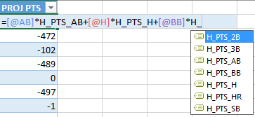 My final formula is:
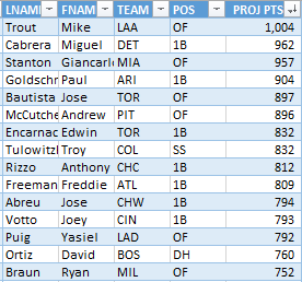
 Hopefully you’ll find that the players come out in an order that seems appropriate given your scoring system (does Mike Trout come out near the top?).
 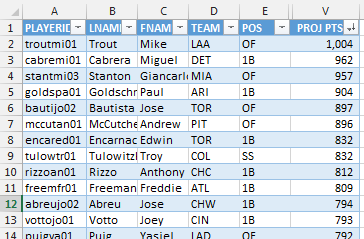 Now let’s move on to the pitchers.
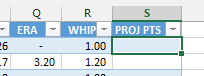 Recall that we named our pitching point values using a “P_PTS_” prefix followed by the abbreviation for the stat category.In my example league, the pitching point values have the following names in Excel:
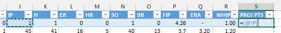
 Excel should recognize the name you’re typing and present you with a list of named cells which follow that pattern. Once you see this list you can double-click on the desired name, use your arrow keys to select “P_PTS_IP” and hit TAB to choose it, or just continue typing the full name.
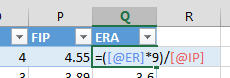
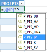 In my scoring system, I want “P_PTS_IP”. Hit enter to save the formula at this point.My completed formula at this point is:
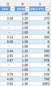
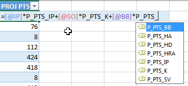 My final formula is:
 Hopefully you’ll find that the players come out in an order that seems appropriate given your scoring system (does Clayton Kershaw come out near the top?).
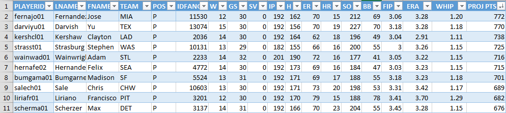

 On the “Home” tab of the Ribbon, select the “Format as Table” drop down and choose a color scheme.
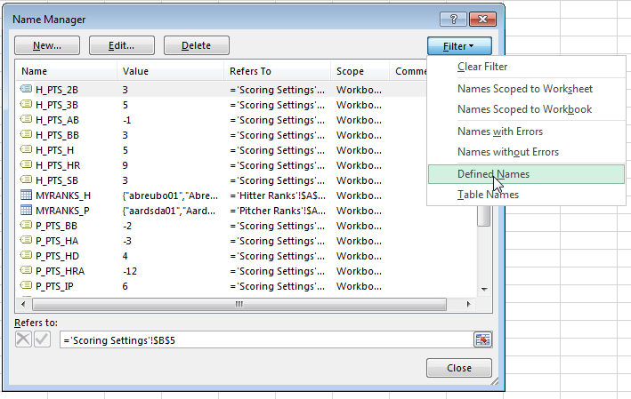
 Locate the only unnamed table (mine is “Table4″ in the example below). Click on the table in the list and then hit the “Edit…” button.
 Change the name of this to “REPLACEMENT_LEVEL” and hit “OK” to save the name. Then hit “Close” to exit the “Name Manager”.
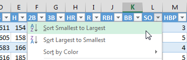
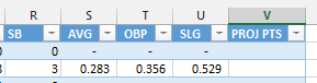
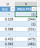
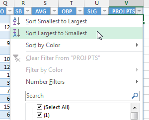
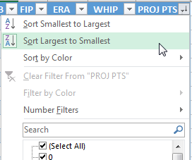
 Use the drop down arrow on the “PROJ PTS” column to ensure it is sorted in descending order (players with most projected points at the top).


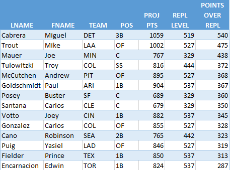
 And type in the projected points for the replacement level catcher into our “REPLACEMENT_LEVEL” table created earlier (e.g. 284 for Rene Rivera).
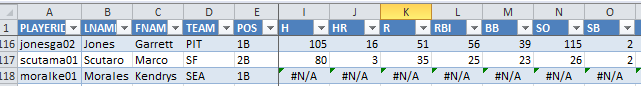
 If you want to be more precise, set your filters to show both 1B and 3B at the same time.


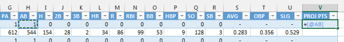
 The formula here will simply be: