Let me come clean. I screwed up. And it likely will cause you to see errors in your spreadsheets. That’s the whole reason for this post.
![Having trouble with VLOOKUP error messages? This post should help.]()
Having trouble with VLOOKUP error messages? This post should help.
What Happened?
While this post is going to address a very important topic (resolving VLOOKUP errors), there wasn’t much of a need for this until I came up with a new format for the Player ID Map. The intent was to make the Player ID Map easily updatable. I hate having to lookup the IDs, birth dates, and handedness of all the new players.
And it’s always bothered me that there was no easy way for you to get updated Player ID information.
Let’s be honest. It’s a pain in the ass. Especially this time of year when players are switching teams every day and minor league players we haven’t had to deal with in the past are now projected to reach the big leagues this season. It’s tedious to keep teams up-to-date and to add these new players.
I needed to find a way to improve this process and to make everyone’s lives a little easier.
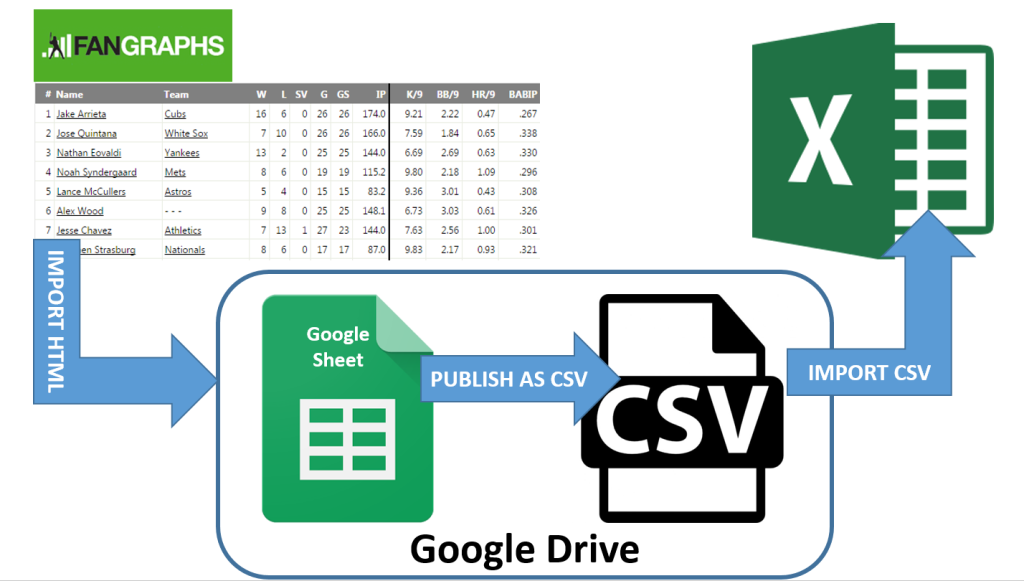
The Solution
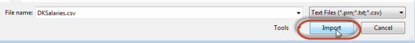
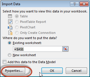
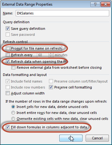
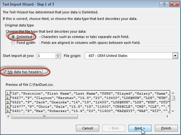
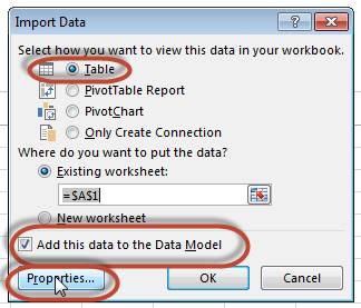
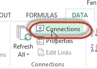
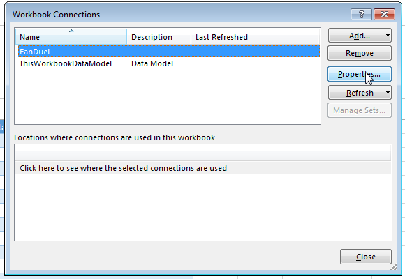
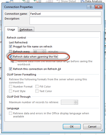
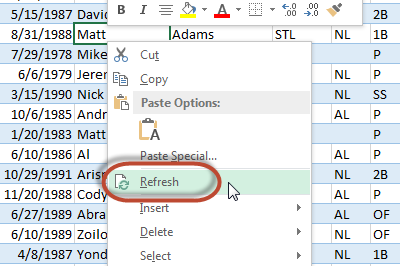
The solution was to make the Player ID Map available in an online CSV file. One you connect that online file to your Excel spreadsheet, you simply have to right-click on the Player ID Map and hit “Refresh”. You will instantly get any update I’ve made.
Sounds amazing, right?
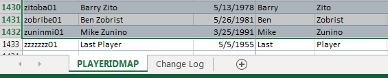
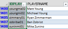
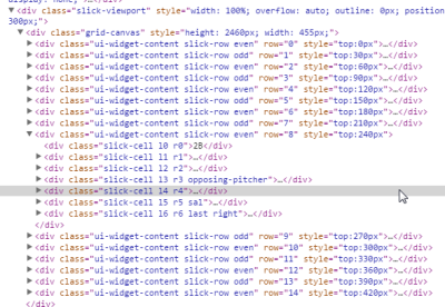
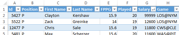
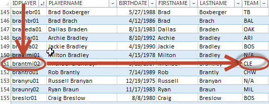
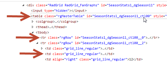
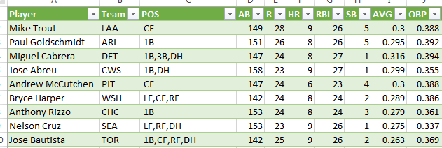
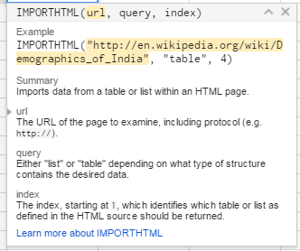
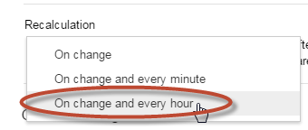
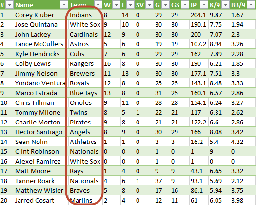
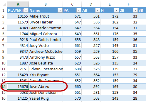
![Major leaguers have a purely numeric Fangraphs ID while minor leaguers have text in their ID.]()
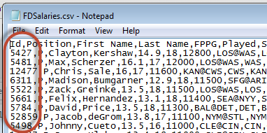
Major leaguers have a purely numeric ID while minor leaguers have text in their ID.
The Problem
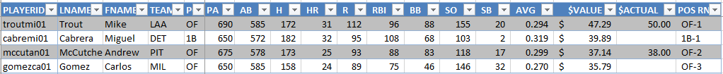
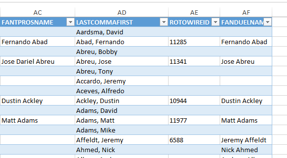
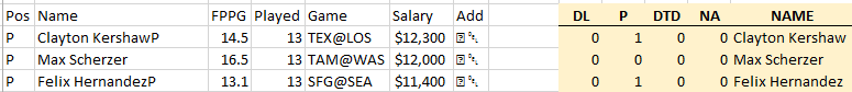
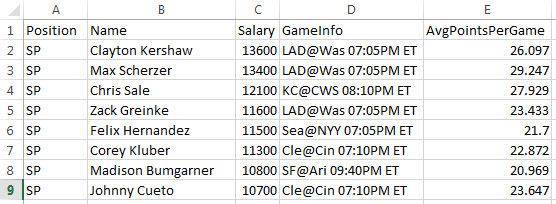
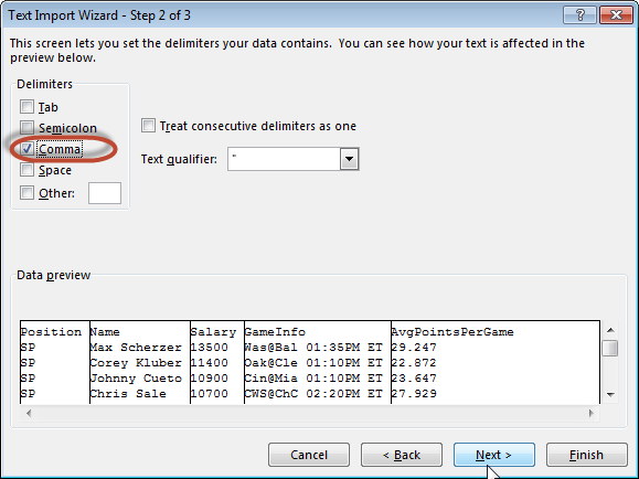
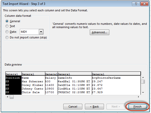
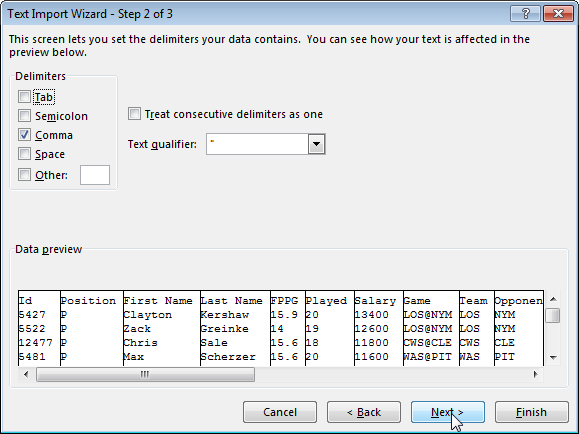
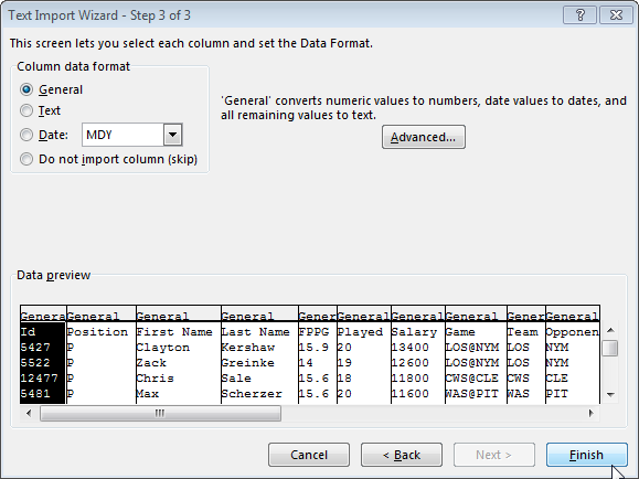
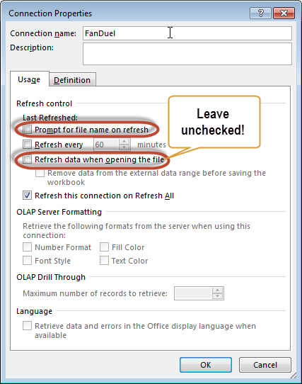
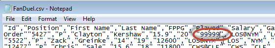
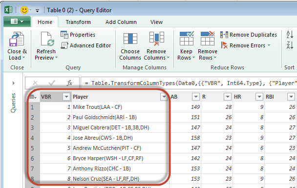
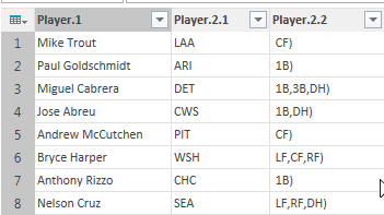
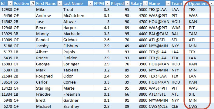
The fly in the ointment happens to be the way Fangraphs structures their player IDs. Major leaguers, like Jose Abreu, have a purely numeric ID. Whereas minor leaguers that have not reach the big leagues, like Yoan Moncada, have the text “sa” in front of a string of numbers.
The unintended consequence of importing the Player ID Map file is that because some IDs contain text, Excel will treat the ENTIRE imported column as text.
The problem is that reports you download from Fangraphs and then open in Excel treat the player ID column as numeric values.
Warning… It’s About to Get Technical
If you’re fine with the old Player ID Map and the fact that it doesn’t get updated very often, you don’t have to use the new one. The old one can be downloaded here and will still be updated periodically. You can stop reading this post and save yourself some sanity.
But if a little complication doesn’t scare you off and you see the value in being able to refresh the Player ID Map and get regular updates… Keep reading.
Text and Numbers Are Treated Differently
Excel and most other computer applications treat text and numbers differently. And this is a common problem with VLOOKUPS. So the number “15676” is not the same as a text string of “15676”. So in our VLOOKUPS, we need to make sure we are comparing numbers to numbers and text to text.
Consider the Error Message
The first step in resolving a VLOOKUP problem is to understand the error message you’re seeing.
The “#N/A” error is the most common VLOOKUP error. And it essentially means that a match was not found during the lookup.
There are two main reasons a match would not be found:
- The item (player ID) doesn’t exist where you told Excel to look for it
- Or you told Excel to look for the wrong data type (look for a text value in a list of numbers, or vice versa)
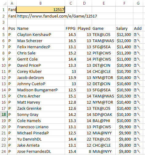
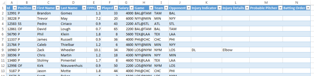
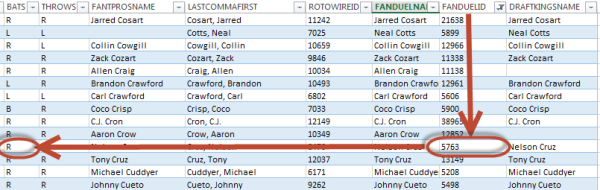
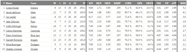
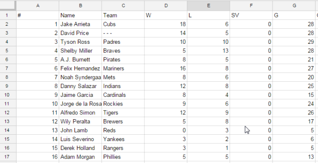
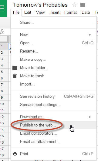
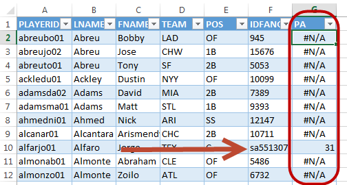
![These are the downloaded Steamer Projections. Abreu's ID is the there. It's in the first column. Why isn't the VLOOKUP finding this???]()
Abreu’s ID is the there. It’s in the first column. Why isn’t the VLOOKUP finding this???
You can easily test the first error by manually performing the search yourself. Let’s walk through a hypothetical example with Jose Abreu. He’s a well known player. He’ll surely be in the Steamer projections I’ve downloaded.
I see from the data that Abreu’s Fangraphs ID is 15676. If I trace that through into the Steamer Hitter projections, I am able to locate Abreu. So why isn’t the VLOOKUP finding the same match?
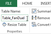
Check Your Formula
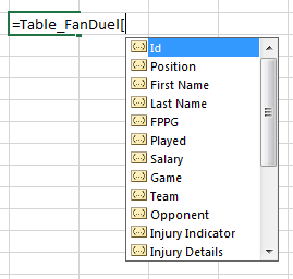
Now that you’ve verified the ID exists, check your formula to make sure it’s performing the same search you did manually. This is another reason I am a big fan of using table names and structured references in Excel, especially when setting up lookup formulas. If you look at the formula below, you can make pretty decent sense of it.
![DOUBLE_CHECK_FORMULA]()
It says to use the value in the “IDFANGRAPHS” column and look for its match in the first column of the “STEAMER_H” table. Then after you find the match, bring back the value in the “PA” (plate appearances) column.
At this time it’s important to revisit the main weakness of the VLOOKUP. The data you’re hoping to match up has to be in the FIRST column of the data set. So when you tell Excel to look in the “STEAMER_H” table, your player IDs have to be in the first column of that table.
That formula looks good to me. You can see from the image above that the PlayerID column is the first column. So we’re confident our formula looks good. Then we may be experiencing the other reason for a VLOOKUP failure – perhaps we told Excel to look for the wrong data type.
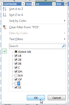
Things to Look Out For
Here are some clues you can look for to determine if you have a data type problem.
Fixing Your Lookup
Now that we’ve identified the problem, how do we go about fixing the data? Or fixing the lookup?
If you are lucky enough to see the green error triangle, you may be able to use Excel’s built in tools to quickly convert numbers being treated as text back to straight numeric values.
To do this, select the first item in the column with the green triangles. Then hit your SHIFT + CTRL + DOWN ARROW KEYs together. This should select the entire column. Then look for the same error warning and choose the option to “Convert to Number”. ![CONVERT_TO_NUMBER]()
Sometimes this works. But this is not the most reliable approach. You won’t always see these triangles. And it can be difficult to resolve even when you do. The best bet is to be able to force the issue by being able to convert a numeric item into text and vice versa.
Excel Formulas to Convert Numeric and Text Data
Fortunately, Excel offers formulas that let us explicitly state that we want something to be treated as a number or treated as text. I think there are more ways than one to do this, but we’re going to look at using the VALUE and TEXT functions.
VALUE
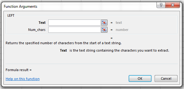
The VALUE function converts a string of text into a number. The string must be numeric in nature, but is treated as text by Excel (this just means you can’t convert the word “four” into a number, it can only convert the text “4” into a number).
The formula requires only one input, the text to be converted.
VALUE(text)
![VALUE_FORMULA]()
text – This can be a text string in quotation marks or a reference to a cell that has the text to be converted.
An example might be a player ID like Jose Abreu’s, “15676”. If we have a feeling that “15676” is being treated as text, we can convert it to a number using the formula =VALUE(“15676”).
TEXT
The TEXT formula is the reverse of VALUE. It converts a number into a text string (assuming the string is composed of numbers). The inputs of the formula are:
TEXT(value, format_text)
- value – This can be a numeric value or a reference to a cell containing the numeric value.
- format_text – a way for you to format the value after it has been converted to a number. Examples of things you can do are to show decimal places, thousands separators (commas), dollar signs, and more.
![TEXT_FORMULA]()
Enough Chit-Chat, Let’s Get to an Example Formula
Alright. Let’s go back to our Jose Abreu example. We’ve double-checked our formula. We’re sure he’s listed in the projections. But we’re still getting an error.
Here’s the current VLOOKUP formula (this should look familiar to you if you’ve followed one of my rankings processes before):
=VLOOKUP([@IDFANGRAPHS],STEAMER_H,COLUMN(STEAMER_H[AB]),FALSE)
Forcing Text to be Treated as a Number
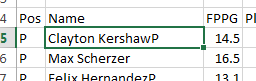
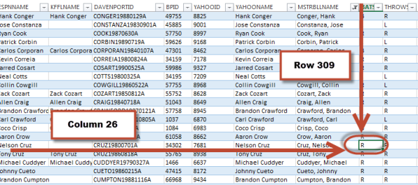
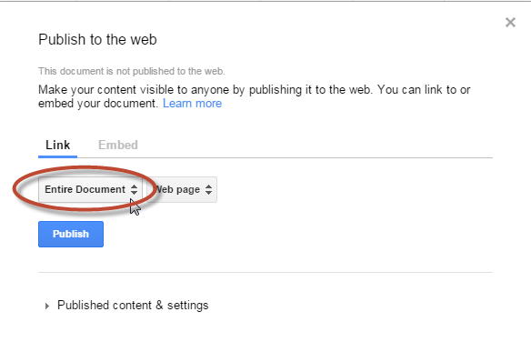
![The IDFANGRAPHS column is left aligned, indicating it's text. Let's try forcing it to be a number.]()
The IDFANGRAPHS column is left aligned, indicating it’s text. Let’s try forcing it to be a number.
Taking a closer look at the spreadsheet, I see the IDFANGRAPHS column is left aligned. This suggests it’s being treated as text. So if we can force that to be treated as a number, it may resolve the issue. The change to the existing VLOOKUP formula is pretty simple (changes are in red):
=VLOOKUP(VALUE([@IDFANGRAPHS]),STEAMER_H,COLUMN(STEAMER_H[AB]),FALSE)
I’ve just taken the existing formula and inserted VALUE around the [@IDFANGRAPHS] information. This tells Excel to force this to be numeric.
After that edit is made, here’s the updated spreadsheet:
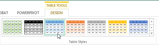
![Many errors disappeared. The #N/A error on an obscure player probably means he's not in the Steamer Projections. But what about the #VALUE! error?]()
Many errors disappeared. The #N/A error on an obscure player probably means he’s not in the Steamer Projections.
But what about the #VALUE! error?
We went from 99% errors to only a few. That’s a good start.
Seeing David Adams, an obscure player, with the “#N/A” error probably just means Steamer didn’t project him.
But the “#VALUE!” error is new. This is Excel telling us that using the “VALUE” formula on a cell that’s not numeric in nature can’t be done. It can’t convert “sa551307” into a number.
Forcing an Item to Be Treated as Text
We can work around the new “#VALUE!” error with the IFERROR formula. I’ve written about this before and you may recall that IFERROR’s power is that it let’s you enter a formula (like a VLOOKUP) and if that formula results in an error, it let’s you control what happens next.
IFERROR is perfect for our situation.
We want to conduct the VLOOKUP first with our IDs being treated as numbers. And if that ends up in an error (#VALUE!), then we want to conduct the same VLOOKUP with the ID being treated as text!
So our formula becomes:
=IFERROR(VLOOKUP(VALUE([@IDFANGRAPHS]),STEAMER_H,COLUMN(STEAMER_H[AB]),FALSE),
VLOOKUP(TEXT([@IDFANGRAPHS],0),STEAMER_H,COLUMN(STEAMER_H[AB]),FALSE))
Before you freak out, this formula isn’t as bad as it looks. Remember that IFERROR can be thought of like this:
=IFERROR(Formula to evaluate,Formula to evaluate if the first one is an error>
And we’re using it this way:
=IFERROR(VLOOKUP with Numeric IDs,Same VLOOKUP but with Text IDs)
The difference is in how we treat the [@IDFANGRAPHS] piece.
To treat [@IDFANGRAPHS] as a number:
=VLOOKUP(VALUE([@IDFANGRAPHS]),STEAMER_H,COLUMN(STEAMER_H[AB]),FALSE)
To treat [@IDFANGRAPHS] as text:
=VLOOKUP(TEXT([@IDFANGRAPHS],0),STEAMER_H,COLUMN(STEAMER_H[AB]),FALSE)
Those are the EXACT same formulas except for the differences in the red font.
But We Still Have Errors!
After making that change we still have the issue of players not included in the Steamer Projections at all. We still see “#N/A” errors. But these are for the obscure players. Not because we have formula issues.
![STILL_MORE_ERRORS]()
To resolve this, we can use IFERROR one more time. We’ll use it like this:
=IFERROR(super long IFERROR from above,0)
This means if a player isn’t found in our “super long IFERROR from above”, then we’ll just see a zero. Here’s the whole formula written out:
=IFERROR(IFERROR(VLOOKUP(VALUE([@IDFANGRAPHS]),STEAMER_H,COLUMN(STEAMER_H[AB]),FALSE),
VLOOKUP(TEXT([@IDFANGRAPHS],0),STEAMER_H,COLUMN(STEAMER_H[AB]),FALSE)),0)
You Made It!
Thanks for making it this far. If you made it to this point, you’re exactly the kind of person I’m writing all this for! I mean that.
What a screw up this turned out to be. I still love the idea of an updatable Player ID Map, so I’m not going to get rid of it. But I also realize this post just got really technical in order to solve a silly problem.
But sometimes that is what it takes. I don’t want to hold back on a topic just because it’s challenging. I’m doing this to help people that aren’t afraid of “complicated”. And in the grand scheme of things, this was probably a helpful discussion that had to be had at some point.
Thanks again for sticking with me. Hopefully you found this discussion valuable. Even if it was caused by a silly mistake.
Please Follow Me on Twitter


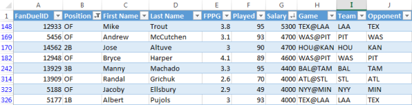
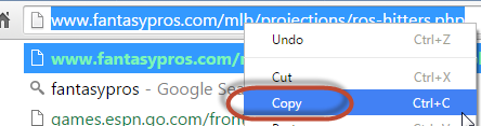
 Copy this information and go to your “Hitter Ranks” tab and paste it into the first cell below the header in column A there.
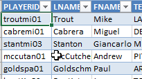
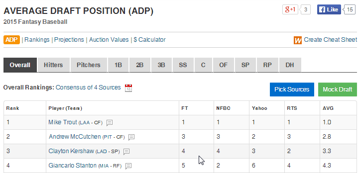


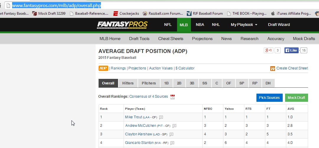


 Use your mouse to select the new “Mike Trout” name we just created. Then hover your mouse over the little black square on the lower right hand corner. You should see the cursor turn to a cross or plus sign. Click your mouse and drag this down for as far as the ADP information goes on the spreadsheet.

 Then click the “Format as Table” button


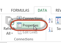
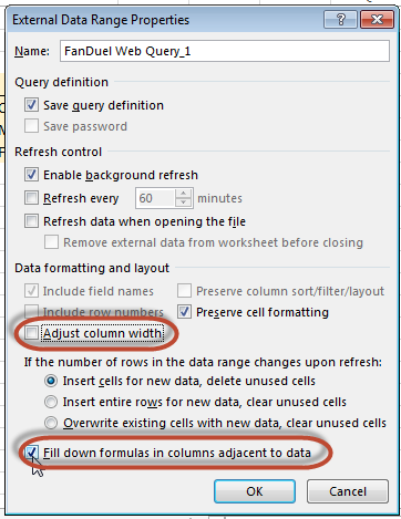


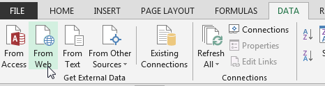
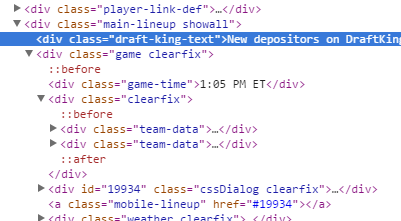
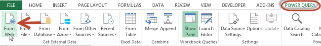
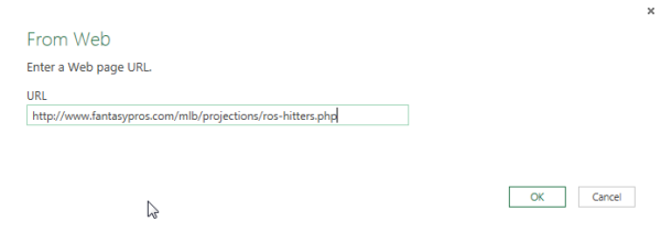
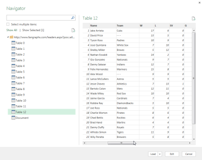
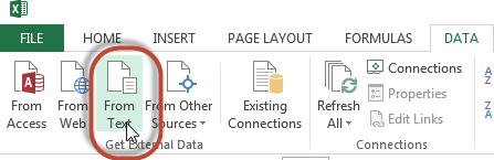 You might remember in the previous web querying article that we used the “From Web” option to “Get External Data” into our Excel files.


 .
. 


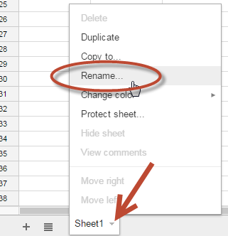


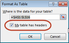
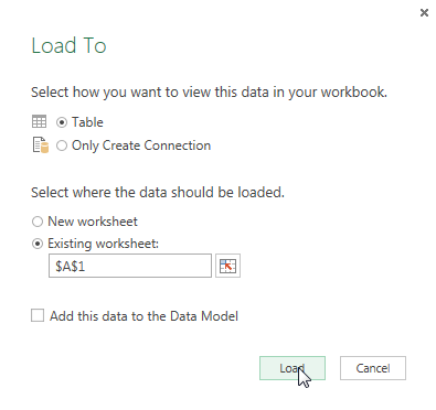
 Then click once to select cell A1. And then click the “Format as Table” drop down menu and choose a desired format for the table.
 Excel should select the table we’ve created. Make sure the “My table has header” box is checked and click “OK”.